Closing the Gender Gap on Wikipedia: Results from Some Simulations

Note: this post has been edited from the original to reflect initial feedback. Most notably, the introductory framing has been changed to focus more on the gap itself and closing it. The second change follows the comment from nemobis. The post now makes the distinction that this analysis only refers to the English Wikipedia.

Introduction

There is a large gap in the number of men and women who contribute to Wikipedia. Researchers have been studying the gender gap in participation between men and women on the website since at least 2007 when it’s usage exploded to tens of thousands of editors.  Most of this research has been on the English-language Wikipedia and the results have consistently shown that the ratio of male to female editors has been at least 4 to 1 since 2007.  Furthermore, recent statistics suggest the gap as only increased since that time.  The gender gap includes not only who edits Wikipedia, but also in the number of edits men and women make, whose contributions persist in articles and whose get deleted, and how long someone remains an editor on Wikipedia.  These numerical differences have arguably contributed to a number of systemic biases in the encyclopedia including imbalances in the topics represented in the world’s encyclopedia, its inapproachable design, and an often hostile editorial culture.

In this post, I simulate the effect of different strategies that can be used to reduce the gender gap on the English Wikipedia.  First, I look at increasing retention among new and existing female editors.  The results indicate that this is a difficult if not impossible approach because of the large gender gap among first time editors.  Second, I look at whether increasing the number of new female editors could close the gap by increasing the pool of first time female editors.  The results are slightly more positive here but, even in this, drastic changes would have to be made to Wikipedia as it is.  Overall, the results indicate that incremental changes to these areas of English Wikipedia are woefully incapable of bringing gender parity within the next decade.  At the end, I discuss some policy solutions for Wikipedia and highlight three desperately needed areas for further research several commentators have noted.

Analytic Approach

I simulate monthly population replacement for active editors on the English-langauge Wikipedia over the next ten years.  The general formula I use for monthly active editors is: last month’s editors * editor retirement rate + new editors * new editor retention rate = current month’s editors.  I take estimates of these parameters, especially as they differ by gender, and predict how large the gender gap will be over the next ten years if we vary editor retention or editor recruitment.  First, let’s start with the current numbers:

Monthly Active Editors: 35,000, 28,000 male + 7,000 female editors

While 125,000 people edited the English Wikipedia last month, few are considered active editors.  Active editors are typically calculated as those who make more than 5 edits in a month.   Last month, Wikimedia statistics counted 33,000 active editors in March (roughly 26% of all editors). For my projections, I round it to 35,000 since I like round numbers and it doesn’t matter for the overall point as we’ll see.  Now, the number of male and female editors is unknown, but estimates range between 9 and 23 percent.  The best estimate is 23% but it’s dated to the height of Wikipedia’s editing which likely over-estimates the prevalence of female editors who have lower retention rates than male editors.  Again, rounding to 20% makes the numbers easy to consider and provides a bit more optimism to this generally dim story.  So, 20% of 35,000 is 7,000 female editors and 35-7 = 28,000 male.

Monthly Retiring Editors: 2.1%

A study done in 2009 found that active editors on English Wikipedia remained active over the course of a year at a rate of about 75 to 80%.  This number is likely to be lower as the researchers found that more recently recruited editors have higher attrition rates than editors who joined the English Wikipedia earlier.  I divide 25% by 12 to turn the annual estimate of 25% loss into a monthly estimate and get a monthly rate of retiring editors equal to 2.1%.  Another way to say this is that 97.9% of active editors are expected to be active next month.

Monthly New Editors: 1200 women with a 7.98% retention rate and 4,800 men with a 10.5% retention rate.

The rate of new editors actually involves two parameters: the number of new male and female editors and the rate at which new users remain on English Wikipedia.  Going back to Wikimedia statistics, there were 6,600 new English users in March.  I round it to 6,000.  Re-using the 20% female statistic from earlier (also generally confirmed among new editors here), this gets us 1,200 new female editors per month and 4,800 new male editors.

An earlier paper found a retention rate of roughly 17% and 13% for male and female editors on English Wikipedia (if I’m reading Figure 4 in the paper correctly).  However, this is higher than the 10% reported by the earlier editor retention study on Wikipedia.  To translate this gender inequality into a estimate of current inequality, I used the .13:.17 ratio to estimate the percent of new female and male editors retained required to produce a 10% global overall average.  Long story short, I estimate new male editors stick around at a rate of about 10.5% and new female editors stick around at a rate of about 7.98%.

So, for male editors in a given month, the formula is: past month female editors*.979 editor retention+4,800 new males * .105 new male retention

For female editors in a given month, the formula is: past month female editors*.979 editor retention + 1,200 new females * .0798 new female retention

Hypotheses

1. Increasing the rate at which new female editors are retained will increase gender parity, bringing the gender gap in monthly active editors to parity by 2016.
2. Decreasing the rate at which existing female editors retire will increase gender parity, bringing the gender gap in monthly active editors to parity by 2016.
3. Increasing the number of new female editors will increase gender parity, bringing the gender gap in monthly active editors to parity by 2016.

Results

New Editor Retention: Editor retention and engagement are big issues for Wikipedia in general and especially for Wikipedians interested in closing the gender gap. A range of things have been attributed to the weak editor retention including the culture and bureaucratization.  The results here indicate that retention is not an easy solution.  In the figure below, I project the percent of monthly users who are female through 2026.

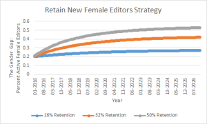
The blue line representing a 16% retention rate for new female editors is what happens to the gender gap if we double the rate at which new female editors become monthly active female editors.  Doubling our effectiveness closes the gap 14 points from 20% women (a 60% gap) to 27% women (a 46% gap) over the course of a decade.  The orange line represents a quadrupling of our current efficacy and, in a decade, gets us to 40% female editors, a 20% gap.  Finally, the grey line represents retaining half of all new female editors closes the gap in a little over five years.  Unfortunately, English Wikipedia has never had a retention rate over 40% according to the editor retention study.

Existing Editor Retention:  Currently, about 25% of editors retire every year or about 2.1% per month.  In this simulation, we ask what happens if we were to increase the retention rate of existing female editors to 80%, 90%, or 100% while maintaining the existing retention rate for male editors at 75%.

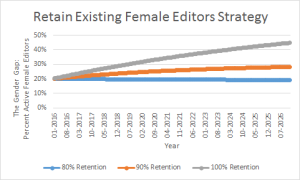
The results are less optimistic than we’d like.  Even if every current and future active, female editor continued editing for the next ten years, the gender gap would still be 10% (45% of editors would be female).  Less extreme changes like increasing current female editor retention to 80% or 90% (which does occur among editors who joined in the early 2000’s and remain on English Wikipedia today) would do little to nothing to close the gap.

More New Female Editors:  The final way to resolve the issue is by increasing the number of new female editors each month.  The results here are somewhat more promising, but demonstrate the same general need for radically different practices.

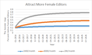
The blue line represents a doubling of current effort from recruiting 1,200 new female editors per month to 2,400.  In 10 years, that gets a monthly editor base that’s 27% women (a 46% gap).  If we quintuple the number of new female editors per month to 6,000, slightly more than the number of men currently recruited, this results in a 47% female editor base in 10 years.  Note, this means that if we achieve gender parity among new editors today, we still would not achieve gender parity among all editors within 10 years.  The last curve is a fantastical one based on assuming Wikipedia recruited women at the same comparative rate it recruits men (4,800 is 20% of 24,000, I rounded in the graph).  In this radical case, parity is reached in one year.

Discussion

These numbers are meant to put into perspective the different levers at Wikipedia’s disposal to address the basic numerical problem of the gender gap.  The results are striking in how difficult the issue of climbing out of gender disparity will be and the kind of radical change that would have to be made to see it happen within the next decade.

That said, there are several things I leave out.  The first has to do with re-recruiting retired users.  One parameter I don’t include in the model is the number of users who used to edit who return to editing in a given month.  Given the historical gender disparity, we can assume that pulling from this pool offers the same issues of recruiting from a largely male-dominated pool.  A second parameter is the ratio of editors to new editors.  I mentioned that 125,000 people edited English Wikipedia last month, but only 33,000 could be considered active.  If the rate at which these drive-by editors could be increased among women, then this may accomplish what the “Recruiting New Female Editors” strategy suggests.

The second and more problematic issue is spillover. For example, more likely than not, you cannot increase the retention rate of women without also increasing the retention rate of men.  Whatever you do to encourage editors to edit will just as likely encourage male and female editors.  Similarly, advertising to female-dominated venues will likely increase the number of male editors recruited as well.  The simulations therefor are unrealistic, best-case scenarios for any strategy targeting only women.

Policy Implications

I want to interpret these results as policy priorities.  The first of which is the scale of the solution needed to make any serious dent in the gender gap.  Any real attempt to close the gender gap has to involve radical action.  I call it radical because, as per the simulations, either the retention rate or the new editor recruitment rate would have to be higher than they have ever been in the history of Wikipedia every month for the next ten years just to close the gap in the next decade.

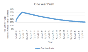
One positive result, indicated by the grey line in the third chart (24,000 new female editors a month), is that the gender gap can be closed within a year if a large, concerted effort is made to recruit new female editors.  My first recommendation then is that there should be a large-scale effort to recruit 24,000 female editors per month.  The figure below plots the simulation.  A short burst of large-scale recruitment could end the gender gap in a year.  If we stop the recruitment once Wikipedia hits 50% and assume retention rates and the gender disparity in new editors returns to what they were are now (which I believe they would change), it would take ten years for the gender gap to return to its current level.

Finally, one issue I do not address is how quickly the gap would close if we combined strategies and both increased the number of new female editors and increased new editor retention.  This is a viable alternative and one whose success can be inferred from the analysis.  Increasing new female editors to gender parity (4,800 female editors) and quadrupling new editor retention (to 32%) would close the gender gap in about three years.  I believe a combination of increasing retention and increasing new female editors is a viable option.  Underlying this whole discussion is a question of whether it is easier to increase retention or increase new monthly editors.  As evident from my recommendation above, I believe increasing new editors is much easier than retaining existing ones.

The solution to optimizing a strategy lies in understanding what is easier or more feasible. Can Wikipedia increase the number of new female editors four-fold and increase new editor retention four-fold every month for three years? Or, can Wikipedia increase female editors by 2,000 times to 24,000 per month for one year?  Or, can it increase editor retention 6 times to 50% every month for the next five years?  The trade off is the cost of sustaining increases in retention versus new editor recruitment every month.

The ultimate question is what will it cost (in terms of money, time, and especially good-will) to increase these rates and how long can Wikipedia sustain that cost?

Future Directions

Based on a range of feedback from several early readers of this post, I’ve decided to mention what the next steps in this estimation should be.  The goal of these next steps is to understand the ecology of editors and the current, historical, and global rates at which editors of different genders transition to different types of editing.

First, one correspondent suggested that only a few hundred editors are needed to change the culture of English Wikipedia because of how densely and socially important its core project organizers are. For me to understand this numerically, I believe we should try to identify these users statistically and determine their trajectories into the core.  The question is where the core users come from and how often they retire.  This is part of the larger question of how and when users transition from new to active to power-users to retirement and so on.

Picking up on this, another correspondent suggested that retention rates have changed such that my current numbers are much further off than I assume here.  If the gender imbalance of new editors, retention rates, and retirement rates have all changed in the direction of increasing the gender gap, my estimates would be very far from current reality.  A historical analysis amounting to an updating of the editor retention study is thus strongly recommended.

Finally, the first commenter notes that all of this applies to English Wikipedia and this is a very astute observation.  I focus on the English Wikipedia because the research on gender and retention rates has already been done.  Thus, I can run numbers rather than first having to find them.  However, the analysis I suggest of repeating the editor retention study and understanding the ecology of users should be replicated for each major language Wikipedia to not only understand the ecologies of users and gender gaps in those communities, but also as a starting point for a more global understanding of the different kinds of gender dynamics across Wikis.

The End of the Career as a Stage in Life?

I’ve had several conversations and read several pieces across the web on changing careers, preparing for retirement, and generally, what we’re supposed to be doing with our working lives.  I’m an intern and full time PhD student, so I’m still in the highly fluid state of an early career.  But, I’ve learned that usually, around this time, people begin to settle into what becomes their “career.”

The career is an odd thing really.  It’s the product of the need for job security for individual employees and a part of the corporate bargain (typically with unions) to take care of the worker in exchange for dedicated service.  It’s protection from at-will work typical of piecework, temp work, support work, and other forms of what is now called “precarious labor” and is a luxury of sorts for the middle and upper-middle classes and some members of the working class.  The classic career was built on tenure and guaranteed by the pension.  So long as you gave several decades of your life to a single company, that company paid for you to live the last decade or two of your life without the need to work.  Today, tenure doesn’t guarantee job security and few people have pensions.  The bright side of this is that the golden handcuffs are much looser than they were ten or twenty years ago.

Everyone with a decent-paying job knows the golden handcuffs – feeling locked into a job or company because the pay and benefits are too good to give up, even if you hate the work.  With the demise of pensions and decreasing importance of tenure, workers’ material ties to an organization do not increase over time like they used to.  At the age of 50, you can move to another job and take your retirement with you.  If you’re moving into a job/career that you’re good at or that’s in higher demand, you may even earn a higher income.

What this means is that the people riding out a job, feeling like they threw their lives away, or who say that work is a sacrifice you make to live the life you want in retirement; are less and less able to justify that perspective.  It’s not that these feelings have gone away.  It’s that workers are not as locked into a job like they once were.  Right now, many people are discovering this in the middle of their careers.  However, I find few young people (including myself) or mid-career people who see themselves changing directions when they’re 45, 50, or 60.  But, there’s less and less reason not to start thinking about it and more and more reason to start planning for it.

Right now, the (middle-class western) life course is to go to college, get married, have kids, settle on a career, retire.  If we were to put ages to these, they would be something like: 18, 24, 27, 35, 65.  Notice how there’s thirty years between the time one starts a career and then retires where nothing is supposed to change in the life course (not so oddly enough “the mid-life crisis” occurs in the middle of this).  In part, this is an artifact of the career system whereby the same thing is supposed to happen for thirty years.  (For those who say a lot happens in those thirty years, you’re right.  But seldom are promotions, vacations, children’s graduations, or personal accomplishments as life-defining as going to college, having children, or getting married.  That’s what makes these ‘stages’ in the life course. Things like divorce happen, but they’re not ‘supposed’ to happen.)   In a sense, when we signed up for the career with a pension and tenure ladder, we created a thirty year period of stasis.  As those supports have gone away, we now have an opportunity to rethink how we want to live our lives during those thirty years.  In a sense, we now have an extra thirty years to define and redefine our lives in the same fundamental ways that we did with school, marriage, our first professional job, and children.

If you’ve followed me up to this point and agree that moving the 401k and finding better, higher paying jobs in your 40s and 50s is possible, the question now is: what do you want to do with your extra 30 years?

I do feel the need to assuage hiring managers (and economists) that the idea of such worker mobility is actually a good thing.  And, I don’t think I have to say much.  While replacing an employee is expensive (several thousand dollars in replacement costs, lost wages’ worth of work, and lost value in expertise) no one wants an unproductive or under-productive employee who isn’t engaged in their work – the employee who rides out their tenure to retirement or who only skirts by with the minimum.  (Actually, few people work like this.  People generally hate being bored and feeling like what they do is meaningless for very long.  We’re good at finding meaning and energy in co-workers, family, or something else and bring that into the job).  But, in a society without careers, employees are increasingly making an active choice to work in a particular job with a particular company.  If employees can move more frequently and define their lives in such flexible ways, those who stay are those who want to be there.  The premise of employee engagement, as consultants are so quick to emphasize, is exactly people’s ability to regularly affirm themselves through work.

So, as work becomes more flexible with the decreasing role of tenure and flexibility of retirement savings, we may want to consider getting rid of the idea of a career as we’ve conceptualized it.  In this increasingly flexible world, we’ve been given an extra thirty years (or a full 1/3rd of our lifespan) to redefine ourselves.  What would you do with all that time?

2N Analytics – Why More Data is Never Enough

The fervor over big data has largely focused on the number of data points now at our disposal by which ever-more specific and powerful analytic insights can be made. But managing the amount of computations is not the biggest challenge.  The biggest challenge is what I call 2N Analytics – creating knowledge within the proliferating data that can be analyzed.  As I’ll show, even very small data is still impossible to compute.  The challenge now, as it has always been, is in developing analysis and knowledge without the ability to compute it all.

In computer science, there are a class of problems called NP-Complete problems.  These are problems where the computations would take such a long time to perform that doing them at a useful scale would be computationally impossible.  One such problem is finding cliques in a network.  (Cliques are groups of people or nodes in which everyone is connected to everyone else.)  To solve this problem, you have to literally check every possible combination of connections between nodes to determine whether the nodes are mutually aware of one another and the group.  Mathematically, this requires 2^N computations where, for every nth node added to the network, the number of computations increases by a power (it’s actually (2^N)-1, but I’m rounding here).  In a network of three people, a computer must do 2^3, or 8, computations.  In a network of just 300 nodes, the computer must do 2^300, or 2×10^90, calculations!  Just for reference, it would take IBM’s Sequoia supercomputer, the fastest we have, 6×10^73 seconds to compute, which is well over 4 times as long as the universe as been around!

Big Data presents the same problem, but not because we have 50 million data points.  Instead, we have 50 million data points across 300 dimensions.  In the same way that clique detection is NP-Complete, so is high dimensional data analysis.  For every new dimension added to data, the analytic possibilities increase at 2^N.  If we just have two dimensions, say cost and sales and we’re trying to predict future earnings, we can calculate the isolated effect of each on profit, the interactive effect of both on profit, and the effects of each controlling for the other.  That’s four calculations for just two variables.  As our number of analytic parameters increases, so do the possibilities for analytic insight grow exponentially.  This is not so new really.  The most widely used social survey, the General Social Survey, collects data on over 1,000 dimension from race and gender to attitudes about the environment and politics.

However, there’s another 2^N problem that does make this problem more salient than ever.  As the number of dimensions grows, our ability to gain meaningful insight from them diminishes because there aren’t enough individual observations.  A basic heuristic in statistics is that, for every variable you put into a linear regression, you need 10-15 observations.  For a regression on 300 dimensions, this is only 3000-4500 observations.  As above, we can multiply the 2×10^90 calculations needed to analyze all 300 dimensions by another 10 or 15.  But, this gets even more mind-numbingly complicated and computationally intractable when we want to do an analysis within dimensions.

Let’s return to the cost and sales example.  Say, you want to compare sales for low-cost versus high cost items.  Knowing your product portfolio, you know that items over $1,000 are your high-end items.  But, though you have 1000 observations, you’ve only sold five items over $1,000 in the past year.  You have a lot of data, but not a lot of data about this fairly rare event.   So, all of a sudden, the two dimensions you can analyze in four ways becomes impossible. Even with 1000 data points because the dimension of interest is too rare.  The thing is, rarity actually becomes extremely common in 2N Analytics and this is a big problem.  Every dimension added actually has at least 2 subdimensions and as many as N subdimensions.  In the case of low- and high-cost items, a 1000-dimension variable is reduced to a 2-dimensional variable (assuming every item costs something slightly different).  This is typically a strength, but when you want to make inferences about specific sub-dimensions (the power of big-N data), the data can run out fairly quickly.

Let’s use an example with the entire U.S. Population.  Using the U.S. census (some of the oldest big data, now containing roughly 300 million people), let’s say you want to investigate the probability of unemployment (7%) for a black (12%) man (50%) in his thirties (13%) in a poor neighborhood (12%) of Detroit (.25%) to a similar man in a similar place in Chicago (1%).  [Note the probabilities here are independent, the unemployment rate for black men in these places is actually much higher. I use these because I happen to know most of the stats off the top of my head.]  Combining these probabilities (.12*.5*.13*.12 = .000936; *.0025; *.01; *.7; x 300 million) you will find that there are 701 such men in Detroit (49 of which are unemployed) and 2889 men in Chicago of whom 202 are unemployed.  In adding five variables, we’ve cut a data set of 300,000,000 people into a data set of 3,500 people of which only 251 have the effect we’re testing.  The power of big-N data is that we still have several thousand people.  But, we still have a couple hundred variables in the American Community Survey (an in-depth survey of samples within the U.S.) we could add to understand the employment likelihood for these two groups of people (political ideology, family, education, transportation access, home ownership, etc.).  Who wants to image how small the data becomes when you compare these 3500 people by their political ideology and family structure?

Hopefully by now, I’ve convinced you that these computational problems are not solved with bigger data and faster computers.  Big data has made us better at getting estimates at such a fine-grained level.  But, the scale needed to solve these problems should be considered unreachable.  Instead, the promise of big data relies on analysts and their ability to choose the right features, set up the right kind of data collection, perform the right kind of analysis, and develop the right kind of conclusions.  What is new is neither the data nor the computers, but our capacity to analytically and computationally engage in reducing these 2N problems to a meaningful and manageable scale from which we can build new insight.

Research Fugue: Measuring Power in Political Campaigns

I’ve been working on a project inspired by the Center for Investigative Reporting and moderated by Kaggle.  I used a network analysis of the movement of money between campaign committees to measure the extent to which different campaigns and different committees were more or less independent, controlling, or broadly influential.  It turns out that corporations have the most broadly influential committees while the most seasoned congressional candidates are the most independent.  However, when you look at the committees that are the most controlling or dependent, things get a bit interesting.  You can download the report and raw results at Influence, Control, Dependent, and Independent.  The code will be up soon.

Doing Program Evaluation Scientifically

I was inspired to write this post after reflecting on James Boutin’s series of posts critiquing the construction and use of data in schools.  There are a lot of ways to screw up evaluations, beginning with misguided initial theories, terrible instrument design, and inept analysis and interpretation.  In this post, I’m not going to tell you all of the ways you can fail and how to succeed.  There are too many for a single post.  Instead, I want to provide the big picture process for doing evaluation scientifically so that you know what you should be getting into when you decide to evaluate.

Evaluation has two components – assessing the causal processes and developing the monitoring system (i.e. benchmarks) to continually assess them.  The causal assessment tells you what about your program and what about your operating environment are influencing your outcomes.  It allows you to say something like, “participation in our interview-skills training program increases the probability of employment by 25%, but the lack of access to public transportation decreases our clients’ probability by 30%.”  The benchmarks allow you to keep track of these influential variables and outcomes and detect any changes or problems with the program.  They allow you to say “over the past year, 50 clients have participated in our interview skills training, but 40 did not have access to public transportation.”  These two pieces of information can play a very influential role in getting city government to expand train or bus routes in your direction or increased funding to pay for bus passes.

My suggestion for a general strategy is to perform a causal analysis once every five or ten years and use the findings to select which benchmarks to track.  This 5-10 year interval is a heuristic.  Some programs operate in very dynamic environments that change quickly relative to other programs.  The more dynamic your environment and the more changes you make to your program, the more often you will have to redo the causal analysis.  In the example above, a new bus line might change the interview program dynamics in several, indirect ways: more clients may come from new areas changing group dynamics, while better access to other resources like a public library or health facilities may improve the job chances of participants but not because of your program.

Causal Evaluation:   Assessing causal relationships is not only the most important part of evaluation, but also the most difficult and most susceptible to bias, misinterpretation, and generally terrible research.  That is why I strongly advise hiring an expert, typically someone who has at least a master’s level training in appropriate research methodologies.  Causal inference involves the highest standards of social sciences research and requires some of the most sophisticated methods we’ve developed (which is why I describe this approach as doing evaluation “scientifically”).  In essence, I suggest paying the $10,000-$50,000 (or more for larger, more complex programs and organizations) once every five to ten years to hire a well-qualified contract researcher or consultant.  My earlier post “Researching With Nonprofits” goes a bit into what this process might be like.  Even better would be to hire one full-time, but I won’t get into the difficulties with financing operating costs.

The most important part of putting the causal evaluation together is the program logic model (for entrepreneurs, this is why you must make one).  Writing out the logic model gives you an explicit understanding of what you believe are the most important processes determining your program’s outcomes and is the starting point for designing the analysis.  Depending on how much data you can gather and to what extent you’re able to randomly select clients to participate in programs, you can expect several waves of data collection or possibly one big one.  Large amounts of data allow for several sophisticated analyses that provide evidence for causal inference.  Small datasets require multiple measures over time to both gather enough data and add temporal variables that help support causal inference.  So, if you’re a small organization or the program is small, you can expect waves of data collection lasting for a period of time determined by the turnover in your program.

So what do you get for your investment?  It depends on the results.  If the study fails to find any significant causal connections and there’s nothing wrong with the data, then a full program review is in order since your program logic model has not received empirical validation.  This is the difference between benchmarks and a causal analysis and why benchmarks are not useful in themselves.  For the interview skills program example, benchmarks would say “40 clients used the service and 30 received a job offer.”  Great, right?  Nope.  The causal analysis concludes that those 30 people would have gotten those jobs without the training.

Benchmarks tell you what’s happening.  The causal analysis can tell you whether you should take credit for it.  The overall goal then is to get the causal part right and then ride on the results for as long as the causal dynamics remain stable.

Benchmarking: If the study succeeds in isolating key causal relationships, then those variables become benchmarks.  To go back to the interview skills program example, if you find that, say, access to transportation, client’s education-level, or involvement in other programs all affect the probability of receiving a job offer, then you collect that information, put it into a spreadsheet, and monitor the changes.  So, if the rate of job offers decreases, you can look and find that your client base in the last cycle was less educated or less involved in the rest of your programs.  Thus, you can say that the program is working with more disadvantaged clients and that you need to do more to get clients involved in other programs.   Hopefully, you can see how this might inspire confidence among your staff and board and encourage donors to open their wallets.

Long-Term Planning:  The basic feature of planning evaluations over time is understanding the dynamics in your environment.  As mentioned above, programs not only have their own dynamics which may change over time, but they also operate within dynamic environments, the causal processes of which will change.  I see three indicators of when a new causal analysis might be necessary.  First, front-line staff and program managers can recognize when dynamics are changing.  Changes in client demographic, new complaints about new issues, or decreasing contact with potential employers can each indicate new dynamics entering the program.  Second, changes in benchmarks can indicate underlying changes in the causal dynamic.  For example, in the interview skills program, if job offers decline, and none of the other measures change correspondingly, it might be time to do another causal analysis.  Finally, dynamics will likely change when you substantively alter your programs.  If you redesign your program to include resume writing or professional writing, dynamics associated with writing like immigration status, race, and education will likely influence how well clients write in your programs and, if the writing component has an impact, the rate of job offers.

Lastly, I would like to take note of current national and sector-level governments, organizations, and thinkers pushing for accountability.  While I believe that data-informed program development and evaluation is the way to go, there isn’t a one-size fits all approach to developing good data and the capacity of organizations to do their own high-standard evaluations represents probably the single biggest barrier to accountability.  Anyone can do research, but to do good research by social scientific standards requires specific training in hypothesis testing, data collection design, and data analysis.  If the accountability movement wants to succeed, it needs to develop the financial and technical resources necessary for organizations to develop this capacity.

The Diminishing Power of the Public, Part 1: Nonprofits as Privatization

This is the first in a series of posts on privatization, the decline of public power, and its implications for democracy and the provision of public and social goods.

A common argument among globalization’s flattening earth theorists is the assertion that state power is being eclipsed by capital mobility, international governmental organizations, immigration, and innovations in transportation and communication.  Here, I want to walk through a counter-argument I’m thinking about.  Historically speaking, state autonomy was actually diminished by democratization.  The more proper question is whether or not public power, engendered by democratic processes and public accountability, is diminishing.  I argue that public power is significantly diminishing, at least in the U.S., and being replaced by a multitude of private powers.  The major forms of this privatization are the outsourcing of responsibility for the provision of public and social goods, the encroachment of private organizations on these goods’ provision, and the privatization of public funds.  In this first part, I want to introduce the question of the declining power of the public and elaborate my first argument: that the provision of public and social goods are being outsourced to private corporations, particularly nonprofits.

First, there’s an ambiguity in the idea of state power.  For globalization researchers, the decline in state power is the declining ability of the state to determine its own policies.  The primary driver for many is global capital flight in which, if states choose anti-capitalist policies, multinational corporations will pick up and move.  Hence, states are forced to dismantle welfare, minimize taxation, and deregulate.  While I would agree that state policy is being influenced by global capital markets, I believe that this conception of state power as policy autonomy obscures what state autonomy actually is.  I argue that states generally are less and less autonomous the more democratic they become.  Democratic states are significantly less autonomous because they are fundamentally beholden to the voters, interest groups, and other public groups that shape elections, policy making, and program implementation.  In essence, the decline of state autonomy has already happened for democracies.

The more pertinent change in state power over the past four decades, best exemplified by the U.S., is the increasingly private control of state money and programmatic responsibility.  This is a broader definition of privatization, which typically refers to governments contracting public enterprises like waste management and parking meters out to for-profit companies.  I define privatization as the private control and responsibility for public resources and programs.  Of course, privatization comes with political overtones and I do not mean to take sides as to whether these trends are better or worse for providing public and social goods.  I only mean to hypothesize about its relationship to public power.

Nonprofits as Privatization:  Prime examples of private responsibility for public programs are nonprofits and traditional privatization initiatives.  Some may be surprised to consider nonprofits as a form of privatization, but they are, in fact, privately-operated corporations (that’s what the “c” in 501(c)(3) stands for).  What is categorically significant about this form of privatization is that the implementation of publicly determined programs is not democratically accountable in the same ways as public programs.  Charter schools are a perfect example of the nonprofit form of privatization.  We elect the school boards who oversee our public school systems.  We do not elect the CEO’s who run charter school management corporations.  Some may think this is a specious distinction since charters are overseen by school boards or other state offices (hence they are still “public”).  But, two important differences should be noted.  First, charter schools are granted exemptions from some of the (democratically chosen) rules and regulations governing public schools.  Secondly, the oversight process is at arms length compared with traditional public schools.

The potential implications of nonprofit privatization are surely more numerous than I’ve come up with, but here are some key points.  First, this privatization likely leads to more innovation, at minimum because of sheer organizational diversity and competition for funding.  This diversity cuts both ways, in that some organizations will be much less effective and potentially harmful while others wildly successful.  The key is the competitive mechanisms which ensure that the ineffective fail and the effective survive.  This gets me to my second implication.  The arms-length relationship between democratic oversight and program implementation problematizes the oversight process because inspection and grant reporting, rather than direct management and public reporting, ensure compliance.  While direct management is no panacea for good governance (think state-run institutions for people with mental illness), an annual inspection has little hope of doing better.  This, I believe is the source for the accountability movement in the third sector.

Third, it allows public programs to tap into a broader range of private resources, particularly foundations (this is more apparent in social services like homeless shelters and services for people with developmental disabilities, than education).  The access to private wealth for public and social programs is a double-edged sword.  On the one hand, the depth of private, philanthropic pocketbooks is enormous.  While there are some policy areas that have long thrived on public and private funding (health, education, research, the arts), other areas like mental illness, job re-training, and homelessness have much more fragmented funding histories that have been positively transformed through the development of the third sector.  On the other hand, it has enabled the retrenchment of the state and the decline in public funding for publicly initiated programs.  Access to private resources did not necessarily cause state budgets to continue to be scaled back, but the ability of social and public services to access private wealth has certainly prevented widespread failure in the nonprofit marketplace in the face of declining public funding.

Finally, this privatization may have shifted the onus of civic engagement into professionalized volunteerism and under-informed philanthropy, rather than political action or democratic civic organizing.  This point goes back to the shift in public provision of services from benevolent associations (like the Elks) to nonprofits.  Before the post-WWII era, public and civic resources circulated through communities via politically active civic groups with regular meetings and democratically elected leadership.  There was a marriage of long-term civic engagement, political activism, and community self-help.  Those days are long gone, replaced by short-term, hyper-circumscribed volunteerism in the professional machinery of an albeit virtuously intending corporation.  Individual philanthropy, rather than being donations to your civic group’s democratically-controlled community pot, are determined by friendship networks (“the ask”), entertainment (galas, concerts, and the like), and emotional appeals.  This represents an information poor market driven by social convenience and an appealing narrative, rather than long-term social relationships, systematic knowledge, and democratic control over the use of donor funds.  It should come as no surprise that nonprofit leaders like Sean Stannard-Stockton and nouveau-riche philanthropists like Bill Gates and Pierre Omidyar are so interested in treating philanthropy as a form of investment.  There is wide-spread concern that the philanthropic marketplace is driven by emotions and convenience (and institutionalized traditions among old-school foundations) rather than impact.  As for volunteers and donors, they’ll have to get their democratic community elsewhere.

In conclusion, the increasing amount of private control over public resources and responsibilities, which I’ve broadened to include nonprofits, has significant, if morally ambiguous, consequences.  This shift, broadly speaking, represents a significant decline in the power of the public to control the provision of public and social services.  This nonprofit form of privatization is not, as some may argue, a capitalist take-over of the public sector because the nonprofit sector is categorically not capitalistic (though it is a marketplace).  Other forms of the declining power of the public, however, are capitalistic as I explain in the next post on the encroachment of private enterprises on public services.

Researching With Nonprofits

There seems to be a growing integration of higher education with real world experience.  While internships are the most historically common form, other types of university-community collaboration are emerging with success.  Take campusCATALYST for example.  They are a graduate student mentored, undergraduate consulting outfit for nonprofits.  Their recent projects include a fundraising and marketing plan for an at-risk youth program and designing a product line to provide an independent line of income.  Consulting projects like these are gaining in popularity in business schools and mirror an important part of professional academics.   But, there’s also a growing number of programs for students in the social sciences to develop their research skills by helping nonprofits.  I wanted to share a bit of my experience researching with nonprofits to illustrate how these programs work and what value they can provide to nonprofits and students.

As an undergraduate, I was a part of the Public Service Research Program (PSRP) at Appalachian State University.  App State, like a number of other universities, imported the program from Stanford’s Public Service Scholars Program.  Basically, I spent a year, under the mentorship of a professor, working with a volunteer office to figure out why so few men volunteered there.  The staff and I put together a couple of hypotheses and created a survey to test them.  It turned out that men and women responded strongly to recruiters of the same gender.  Thus, since the office only had a few men, it was more difficult to recruit more men in proportion to women.

Currently, I volunteer my time working on program evaluation with the Neighborhood Writing Alliance.  We set up some basic outcomes we thought were important, given their mission statement and my knowledge of social science research, wrote up a survey, and analyzed the results.  Now, the NWA knows how engagement in their writing work shops connect with their writers’ satisfaction with the program; how engaged writers are in other organizations, their local communities, and politics; and writers’ perceptions of fairness, trust, and self-confidence.  All of this goes into their grant-writing, reports to their board, and program development.

These experiences illustrate the positive potential of combining social scientific education with nonprofits’ research needs.  As a student, these projects have challenged me to put my understanding of social trends and processes to the test.  The most important lesson I learned was getting the input of the people I worked with.  Social scientists do not have a monopoly on knowledge.  Nonprofit staff have good ideas about what’s going on in their organizations and their input is crucial to creating realistic hypotheses and data collection methods.  On the academic side, these experiences have pushed me to explain plainly what sociology is and says and learn about different areas of research like volunteerism and, thanks to an NWA intern, a niche on assessing community empowerment at the boundary between sustainability and psychology.  Finally, and most practically, it taught me to manage a complicated, multi-stakeholder research project.

For nonprofits, the benefits can be just as enormous.  Social scientific methods and research are at the heart of the growing demand for program evaluation and impact assessment.  Further, I’ve found that nonprofits have an incredible range of interesting and very relevant questions from staff training and retention to local food security and health trends.  A good student can do the background research and collaborate in constructing a workable research strategy with the result being a broader, research-based perspective on the problem and, hopefully, an answer (research is never guaranteed to provide actionable results).

Given that 85% of undergraduates in the social sciences go on to work in nonprofits, corporations, and the government; instituting a PSRP kind of program, I believe, not only pushes students’ engagement with the practice of social research, but prepares them to actually use it in their lives after university.  As for nonprofits, such a broad engagement would, among other things, help cover the accountability funding gap where grant-makers ask for evaluations, but won’t pay for the overhead cost of a researcher.

Finally, if you’re a nonprofit looking to find a research volunteer or intern, contact the nearest university’s civic engagement or volunteer office and see if they have a such a program.  If not, encourage them to look into one.  At the very least, they will post your opening and channel an interested student your way.

DonorsChoose Supplement Part 3: Market Corrections

Note: In preparation for the results announcement by DonorsChoose, this series is meant to carve up different issues raised by my work on the DonorsChoose Data and address them directly and more fully.  You can find the original announcement and report at Predicting Success on DonorsChoose.org.

If, based on my findings, we believe that there are some deserving projects that are being unwarrantably disadvantaged, by say teacher gender or metropolitan location or even the state of origin, there are a couple of ways we can use the algorithm to change the dynamics of the market and test the efficacy of those changes.  My philosophy behind this is that, given that the DonorChoose market is biased towards urban schools, for example, if we don’t believe urban schools are any more deserving than suburban or rural schools (see my discussion on deservingness for why this might be true), then I would call that systematic under-valuation in the market.  Using the algorithm, we can test potential correctives for that.

The first intervention was actually suggested to me by Jonathan Eyler-Werve.  He suggested that search pages could weight the search results based on whether they were urban/suburban/rural or by state, for example, such that under-valued projects could be found earlier.  Technically speaking, this random sort would be weighted, such that more rural and suburban projects, randomly selected from those returned by a user’s search, would show up earlier.  So, say that you’re looking to help out a music project that’s coming down to the wire.  You might not care whether it’s urban or suburban, but, as things stand now, the higher number of urban projects in the system means that roughly 60% of the project’s you’ll see will be urban.  You’ll more likely donate to an urban school just by sheer roll of the dice.  With this weighted, random sort, the search results will balance out the proportion of urban, suburban, and rural projects.  Of course, this would not apply to searches that explicitly ask for urban, suburban, or rural projects.  Testing the impact of these corrections would involve re-running the analysis that produced this model on the post-implementation rates of success and seeing whether the significance of the urban/suburban/rural variables decreased.  If the significance decreases, then the bias has decreased.

Another form of market correction, and one which I mentioned in the report, would be allowing donors to see a project’s chances of success or sort their results by them.  This directly informs donors of the value given to these projects by the market and let’s donors decide if the project is really deserving of a 30% chance.  Thus, a donor could look at two similar projects, like two music programs in Chicago, and know that one has a 60% chance of success and the other an 80% chance.  If the donor thinks the first one is actually more deserving, they might be more motivated to donate to it to try and help its chances.  They may even start a giving page around it.  This approach is a donor-driven market correction in which donor’s can use their own set of preferences to determine if the 60% project is really less deserving than the 80% project.

Monitoring the effect of this implementation would involve re-running the model after this has been implemented and testing any changes in the probability of projects.  Thus, if the original algorithm predicted a 60% probability of success and the post-implementation data shows some projects going to 80%, we can see which variables in those projects correlate with the increase in probability.  If we find, for example, that projects posted by female teachers increase in probability, then we can infer that donors are correcting for the existing gender bias.  The same goes for any variable measured.

Finally, offline strategic initiatives can be developed to target under-valued projects.  For example, a foundation focusing on rural development may be very interested in trying to build support on DonorsChoose for rural projects.  Most importantly, this research provides justification for this strategy, in that rural schools are less likely to reach project completion.  Thus, such a foundation might be convinced to offer matching funds to rural projects or distribute gift cards to rural areas to raise awareness of DonorsChoose and build the rural donor pool.  The same goes for under-engaged states.  I’m not sure what the retention rate of gift cards is, though it could easily be figured out from the data provided for this competition.  In the case of a matching funds initiative, assessing the impact would involve the first method mentioned above, seeing whether significance of the rural variable decreased during the fund period.  As for recruiting new donors through gift cards, not only can we assess how many people used the gift cards, but, using the second method mentioned above, we can estimate the lasting effect of the initiative.

If you have any other ideas of how this prediction algorithm might be used to improve the DonorsChoose market, please feel free to discuss it in the comments section below.

DonorsChoose Supplement Part 2: Deservingness

Note: In preparation for the results announcement by DonorsChoose, this series is meant to carve up different issues raised by my work on the DonorsChoose Data and address them directly and more fully.  You can find the original announcement and report at Predicting Success on DonorsChoose.org.

In the report, I argue that donors choose what they perceive to be the most deserving projects.  I explicated this a little in my first supplement, but want to refocus on it here to talk about what deservingness may be and how we might be able to reflect on exactly what deservingness should be.  First though, I dispel the idea of interpreting the data as a straight-forward measure of deservingness.

I found a number of categories that negatively affect the probability of success.  For example, suburban and rural schools, and projects for non-high school students are less likely to reach project completion.  This does not necessarily mean that donors perceive urban high schools as more deserving.  It may be due to the fact that donors are more likely to be parents of urban high school children donating to their child’s school.  From the data provided by DonorsChoose, this hypothesis is untestable.  Thus, my talking about the findings in terms of deservingness is based on an informed, but not fully justified assumption that the findings do in fact, to some extent, come from donor’s notions of deservingness.  Essentially, in light of the fact that there are alternative explanations of the findings, I still believe that some donors see urban high schools as more deserving.

The findings of the report allow us to ask ourselves who is more deserving.  Obviously, the effect of gender, urban/suburban/rural, and subject area are fertile grounds for discussion.  Gender presents a unique challenge, first and foremost, because there is a real question of whether or not donor’s consciously see male teachers as more deserving.  While there is plenty of literature on the glass escalator effect for men in typically female dominated workplaces, whether or not this applies to DonorsChoose is not testable with the data.  It could be that male teachers write different types of essays that donors find more persuasive or ask for different types of resources within given categories.  In essence, the gender variable could be capturing the effect of something else that I didn’t take into account.  This becomes less likely the more, other variables I control for (and I controlled for a lot of them).  Given the previous research on this issue and the number of controls I introduced, I am inclined to believe that the gender effect is actually attributable to a gender bias.  The question then is, is that okay?  Are we comfortable with the idea that male teachers are more deserving than their female counterparts?  I would say not.  How could we fix that?  I’ll elaborate that in the next supplement on strategies for correcting valuations in the DonorsChoose market.

The salience of the urban/suburban/rural distinction on project success raises two issues.  The first harkens back to my earlier discussion of alternative interpretations to deservingness.  I’m inclined to believe that there are more urban donors (by simple dint of population).  The challenge then is to reach more rural and suburban donors.  I’m also inclined to believe that non-local donors,  those who are not fully tied to donating to their local schools, are biased towards urban schools because of the recent education reform movement’s emphasis on urban school reform.  Urban schools are the locus of heated debate about educational innovation (i.e. the charter school movement) and public school reform (i.e. the accountability movement).  On DonorsChoose, I believe this translates into the perception among some donors that urban schools are especially wracked with problems and that their students are especially disadvantaged.  (I also believe this translates into the preference for charter schools that I found).  Educational research is not my area, so I’m not well-versed in the research on whether or not urban schools are more or less disadvantaged than suburban or rural schools (when you control for local property values, parents education, and the like).  Thus, I can’t make an informed opinion as to whether this perception of urban deservingness is justified.  But, if you buy my argument, now that we have evidence that urban schools are preferred among some donors, we can find out if that perception is warranted, and if necessary, try to change it.

Finally, the differential preferences for donations to different subject areas ranked very roughly from most preferred to least: arts, sports, STEM, social science, special education, applied, and language and writing.  There are ways to obtain a more accurate ranking (though this one is likely to be pretty close), but I only want to use this as an example.  If we assume deservingness, we could read these rankings as reflecting a sentiment in which donors believe some subjects are already disproportionately under-funded (i.e. arts and after-school athletics programs), but still adhere to our present emphasis on the value of math and science education (the STEM fields).  But, now that we know how these subjects stand, we can ask, should more be done to promote special education or, applied or language projects?  This would be a good selling point for getting a foundation to fund a campaign for literature projects.  In addition, we can ask ourselves whether or not we should be distinguishing by subject area.  Is a piano for a music program more deserving than microscopes for a biology class?  I believe that when a donor searches through DonorsChoose, they are more likely to say to themselves, “I want to fund the arts because the government won’t,” than say,  “The piano is more important than the microscope.”  In essence, I believe the bias for different subject areas is applied at the beginning, rather than at the final choice between different concrete options.  However, the outcome is the same, the piano is more likely to be funded than the microscope and we have to decide if that’s a worthwhile value judgement.

I’ve gone through just some of the findings to introduce their implications for DonorsChoose and for us as a philanthropic society judging schools and programs based on an idea of deservingness.  In my next post, I’ll discuss some ways we can use the prediction algorithm to fix any biases in the market that we find unjustifiable.

DonorsChoose Summary Part 1: Sociological Insights

Note: In preparation for the results announcement by DonorsChoose, this series is meant to carve up different issues raised by my work on the DonorsChoose Data and address them directly and more fully.  You can find the original announcement and report at Predicting Success on DonorsChoose.org.

Creating the algorithm involved running standard statistical analyses which are typically used for description.  In the original report, I only mention the sociological readings of the data I analyzed.  Here, I want to do a fuller sociological interpretation.

If, like most people, you don’t know how to read a regression table (the appendices in the report), first focus on the sign of the numbers (are they positive or negative).   The price variable is negative, thus, the probability of success decreases for every additional dollar requested (it’s actually a logged price, so it’s not that simple, but that’s the very basic interpretation).  The male variable is positive, thus male teachers have a higher probability of success on DonorsChoose than female teachers.    As for the actual numbers, they are log odds (a result of the particular statistical model).  To make them make sense, just exponentiate them (e^number).  Thus, the male .18360 becomes 1.20, meaning that men are 1.20 times more likely than women to succeed.

Maximizing Impact? The number of students impacted, whether the project would be used by future students, and if the project would be used for essential instruction all had no effect on project success.  These seem to be the most direct measures of impact and it makes me wonder how concerned donors are with maximizing their impact.  In the report, I summarize donors’ as motivated by notions of deservingness, not impact, because of this.  However, this could be due to the fact that this information is at the very bottom of project pages and, except for essential/enrichment, you cannot search by these features.  Donors might care, but not be aware that this information is available or might not be able to use it effectively.

Causation and Correlation: In describing my results in the paper, I talk ambiguously about the link between the significant variables and the probability of success.  While I maintain that, if a teacher posts a proposal for books, they will have a higher actual probability than if that same teacher requested technology, this could be read as a causal claim though it is not.  I do however, claim that receiving matching funds or donations through a giving page do cause an increase in probability.  The reasoning is fundamentally theoretical.  These matching funds and giving pages are real actions that, according to the statistics,  significantly affect the chances of success.

The Power of Giving Pages: The incredible significance of giving pages (increasing the likelihood of success by more than 50% in some cases) is very interesting theoretically.  I believe that active giving pages are sites of highly engaged donors who not only fund projects (as opposed to the 90% of visitors to DonorsChoose who do not), but actively recruit and motivate other donors.  This direct appeal by a highly engaged collection of people is how social movements operate and what sociologists mean when we talk about the power of social networks to create social capital and motivate collective action.

Market Effectiveness: Most often, people talk about markets in terms of efficiency.  I believe the first measure of a market should be effectiveness.  The first question should be whether or not a market is providing the goods it is supposed to to the participants who want them.  For DonorsChoose, are they connecting donors to the projects that they want to fund?  My belief is that they are pretty effective based on the fact that most of their searchable terms (poverty level, subject area, etc.) were also significant variables.  A significant number of donors care whether they’re donating to a music program or a soccer team.  They care whether the money will fund a class library or a new smart board.  Despite the insignificance of the impact measures (which may be due more to their lack of integration in the search system), DonorsChoose allows donors to choose projects based on the dimensions they care about.  There could be a reverse causation here, a market making dimension where donors come to see subject area or resource type as important only because DonorsChoose offers them as potential search options.  This does not negate the inference however that they are significant, only where the preferences come from.

Market Change: In the first version of my report, I stated that the positivity of the Year variable meant that the DonorsChoose market was becoming more effective over time because the probability of success increased every year.  I retract that, because Year was actually not so generally positive across the models.  There are a couple of possible explanations for the declining measures, following simple supply and demand.  I think the most probable explanation would be an increasing number of projects posted.  With more projects being posted every year, if the number of donors does not increase proportionately as well, then the overall rate of success is likely to go down.  The supply of donor funds has not kept up with project demand.  I find the opposite side of supply/demand, a decreasing amount of donor funds, less probable given the growth of activity on DonorsChoose, though it could be driven by the current economic environment.

These are some of the surely multitudinous implications that can be drawn from my research here.  Please feel free to ask questions or posit your own interpretation of what’s going on in the comments section below.